Ultimate Guide to Iterative Imputer and KNN Imputer in Machine Learning (with Manual Examples)

Handling missing data is a crucial step in any machine learning pipeline. Two powerful techniques for this are:

• Iterative Imputer (used in MICE)
• KNN Imputer (based on similarity)

In this blog, we’ll explore both methods from scratch, using easy-to-understand language, manual examples, and real-world use cases. Whether you’re a beginner or someone brushing up, this guide will give you the complete picture.

Why Handling Missing Values Matters?

Real-world datasets often have null or missing values in columns. If you skip this step:

• You lose valuable data by dropping rows
• Your model performance will be biased or poor
• Some algorithms will fail to train or predict

Thus, proper imputation (filling missing data) is critical.

 What Is Iterative Imputer?

Iterative Imputer is a method to fill missing values in a dataset using Multivariate Imputation. It treats each feature with missing values as a regression problem, predicting the missing values based on the other features.

In simple terms:

                                       “Instead of just filling missing values with a mean or median (which is naive), let’s learn what the    missing value could have been by looking at patterns in the other columns.”

Why is it used?

It is used because:

• Simple imputation methods like mean/median/mode ignore relationships between features.
• It can preserve multivariate structure, i.e., the relationship between columns.
• It generally gives better model performance than simple methods when the data is not missing completely at random.

When and Where is it used?

Use Iterative Imputer when:

• You have missing values (NaNs) scattered across multiple columns.
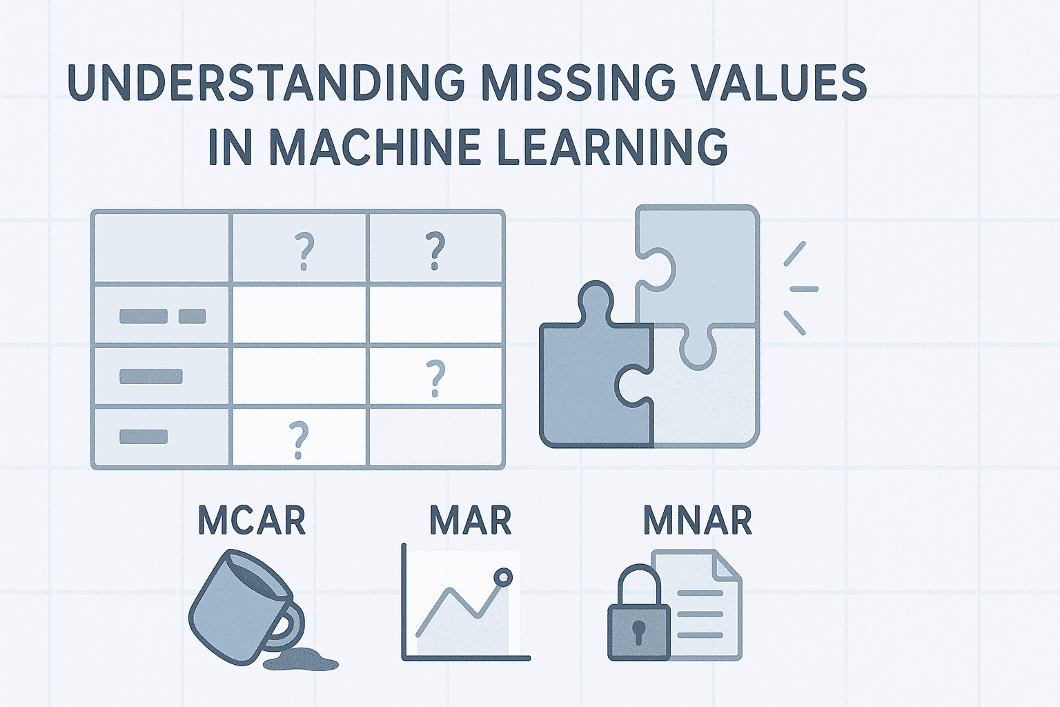
• When missing values type MAR (Missing at Random)
• The columns are correlated or have some predictive power over each other.
• You want to retain as much information as possible rather than discarding rows or filling blindly.
• Especially good in healthcare, finance, real estate, or any domain where columns are interrelated.

 Don’t use it when:

• You have too much missing data (e.g., >50% in a column).
• Features are not correlated at all.
• You want faster imputation (Iterative Imputer is slower than mean/median imputation).

3. How Iterative Imputer Works (Step-by-Step)?

Let’s go through it step-by-step, first conceptually, then with a simple manual numerical example, and finally code.

Steps:

1. Start with a dataset with missing values.
2. Initialize missing values with initial guesses (like mean or median).
3. For each feature with missing values:

• Treat it as a target (y).
• Treat other columns as features (X).
• Fit a regression model on non-missing rows.
• Predict the missing values.

      4. Repeat this process for all columns with missing values.

      5. Iterate steps 3–4 until the values converge or until a maximum number of iterations is reached.

Result:

You get a complete dataset, filled with more intelligent estimates than just mean or median.

Dataset with missing values:

A	B	C
1.0	2.0	3.0
2.0	NaN	6.0
3.0	6.0	NaN
NaN	8.0	9.0

Step 1: Initialize missing values

Let’s fill missing values with column means first:

• Mean of B (ignoring NaN) = (2 + 6 + 8)/3 = 5.33
• Mean of C = (3 + 6 + 9)/3 = 6.0
• Mean of A = (1 + 2 + 3)/3 = 2.0

A	B	C
1.0	2.0	3.0
2.0	5.33	6.0
3.0	6.0	6.0
2.0	8.0	9.0

Step 2: Start Imputation

Let’s say we want to impute B in row 2 (originally NaN).

• Use other features (A and C) to predict B.
• Use rows with complete B: row 1, row 3, row 4
• X (A, C) → [[1.0, 3.0], [3.0, 6.0], [2.0, 9.0]]
• y (B) → [2.0, 6.0, 8.0]

Train a simple linear regression on this.

For row 2: A=2.0, C=6.0 → Predict B

Assume regression model gives B = 5

So, we replace 5.33 with 5.0 (a better estimate based on regression).

Impute column C

• Target: C
• Features: A and updated B
• Predict the missing value in row 3
• Use A = 3.0 and B = 6.0
• Replace C = 6.0 (initial guess) with predicted value, say 6.2

Impute column A

• Target: A
• Features: updated B and C
• Use values from latest imputation for B and C to predict A in row 4.

Iteration Cycle:

This cycle (imputing B → C → A) is done for multiple iterations (by default 10 in scikit-learn), so the estimates keep improving each time.

Each time:

• You use the latest values for the predictors.
• Previously imputed values can be updated again.
• The imputation converges after several passes (no big changes anymore).

Important Notes:

Concept	Description
Initial guess	Usually mean/median imputation
Predictive model	By default BayesianRidge, but you can use any regressor (e.g., RandomForest)
Each column treated as target	One at a time, while using others as predictors
Updated values used	Yes, always the latest values are used in subsequent imputations

Code Implementation:

import numpy as np
import pandas as pd
from sklearn.experimental import enable_iterative_imputer
from sklearn.impute import IterativeImputer
from sklearn.linear_model import BayesianRidge

# Sample data with missing values
data = pd.DataFrame({
‘A’: [1, 2, np.nan, 4],
‘B’: [2, np.nan, 6, 8],
‘C’: [np.nan, 5, 6, 9],
‘D’: [3, 4, 2, np.nan]
})
print(“Original Data:”)
print(data)

# Create IterativeImputer
imputer = IterativeImputer(estimator=BayesianRidge(), max_iter=10, random_state=0)

# estimator=BayesianRidge(), max_iter=10,; >> These parameters are used by default in scikit-learn

# Fit and transform
imputed_array = imputer.fit_transform(data)

# Convert back to DataFrame
imputed_data = pd.DataFrame(imputed_array, columns=data.columns)
print(“\nImputed Data:”)
print(imputed_data)

What Is the Relationship Between Iterative Imputer and MICE?

• MICE (Multiple Imputation by Chained Equations) is a statistical technique for handling missing data.
• It works by modeling each feature with missing values as a function of other features in a round-robin (chained) fashion.
• It repeats this process multiple times (iterations) to refine the imputed values.
• The key idea is to generate multiple imputed datasets, reflecting the uncertainty in missing data.
• After generating those datasets, we train separate models on each, then combine results (averaging, ensembling, etc.).

Iterative Imputer – The Tool

• IterativeImputer is scikit-learn’s implementation of the chained equation technique.
• It works similarly to MICE — it treats each feature with missing values as a regression target, and iteratively fills them.
• But here’s the catch:
  By default, IterativeImputer is a single imputation technique, meaning it gives one completed dataset.

Note: If we run max_iter = 10 for both techniques then Iterative Imputer give only one data set without missing values but MICE give 10 datasets without missing values.

What Is KNN Imputer?

KNN Imputer (K-Nearest Neighbors Imputer) fills in missing values by:

          Finding the K most similar (nearest) rows based on other feature values and then taking the average (or weighted average) of those neighbors to fill the missing value.

It’s a non-parametric, instance-based imputation method.

In simple terms:

“It finds the most similar (nearest) rows based on other columns and uses their values to fill in the missing data.”

When and Why to Use KNN Imputer?

When:

• Missing values are random and not too many.
• Data has patterns — similar rows tend to have similar values.

Avoid when:

• Huge dataset (KNN is expensive).
• Missing data is excessive (>40%).

Step-by-Step Example (Manual Calculation):

Row	Feature1	Feature2	Feature3
A	1	2	3
B	2	NaN	4
C	3	6	NaN
D	4	8	6
E	NaN	10	7

We’ll use:

• K = 2 (2 nearest neighbors)
• Euclidean distance (standard distance)
• Only complete features are used to compute distances

How Distance is Calculated?

For each row with a missing value:

1. Identify rows without missing values in the relevant feature.
2. Compute Euclidean distance between the row with NaN and the other rows, ignoring the missing feature.
3. Select K rows with the smallest distances.

Step 1: Impute Feature2 for Row B

Row B = [2, NaN, 4]

We want to impute Feature2.

We find distances excluding Feature2, so we use Feature1 and Feature3.

Compare with rows that have Feature2 value:

Row	Feature1	Feature2	Feature3
A	1	2	3
C	3	6	NaN ❌
D	4	8	6
E	NaN ❌	10	7

Only A and D can be used (C has NaN in Feature3, E has NaN in Feature1)

Distances from B = [2, NaN, 4]

A = [1, 2, 3] → Features: 1 and 3 only

Distance(B,A)=sqrt((2−1)^2+(4−3)^2​) = sqrt(1+1)​= sqrt(2​) ≈ 1.41

D = [4, 8, 6]

Distance(B,D)=sqrt((2−4)^2 + (4−6)^2) = sqrt(4+4) = sqrt(8) ≈ 2.83

2 Nearest Neighbors: A and D

Their Feature2 values: 2 (A), 8 (D)

Imputed Value for Feature2 (Row B):

Mean=(2+8)/2​=5

Row B → Feature2 = 5

---

Step 2: Impute Feature3 for Row C

Row C = [3, 6, NaN]

We’ll use Feature1 and Feature2.

Compare with rows that have Feature3:

Row	Feature1	Feature2	Feature3
A	1	2	3
B	2	5 ✅	4
D	4	8	6
E	NaN ❌	10	7

Valid rows: A, B, D

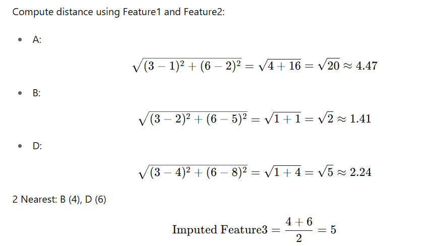
Row C → Feature3 = 5

Step 3: Impute Feature1 for Row E

Row E = [NaN, 10, 7]

Use Feature2 and Feature3 to compute distance.

Compare with rows having Feature1:

Row	Feature1	Feature2	Feature3
A	1	2	3
B	2	5	4
C	3	6	5
D	4	8	6

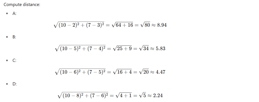
2 Nearest: D (4), C (3)

Imputed Feature1: (4 + 3)/2 = 3.5

Row E → Feature1 = 3.5

Final Imputed Dataset

Row	Feature1	Feature2	Feature3
A	1	2	3
B	2	5	4
C	3	6	5
D	4	8	6
E	3.5	10	7

Imputation Strategy:

• Distance Metric: Euclidean (default), Manhattan, Minkowski
• Weighting: Uniform or distance-based
• k: Hyperparameter to tune (try k=3, k=5, k=7)

Code Implementation:

from sklearn.impute import KNNImputer
import pandas as pd
import numpy as np

#Create the dataset

data = {
‘Feature1’: [1, 2, 3, 4, np.nan],
‘Feature2’: [2, np.nan, 6, 8, 10],
‘Feature3’: [3, 4, np.nan, 6, 7]
}
df = pd.DataFrame(data)

#Initialize KNNImputer with k=2

imputer = KNNImputer(n_neighbors=2)
imputed_data = imputer.fit_transform(df)

#Convert to DataFrame

imputed_df = pd.DataFrame(imputed_data, columns=df.columns)
print(imputed_df.round(2))

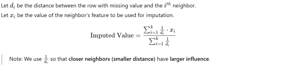
Distance-Weighted KNN Imputation:

Instead of taking a simple average of the K neighbors’ values, we use a weighted average:

• Closer neighbors → get more weight
• Farther neighbors → get less weight

Formula:

Let’s say:

Point	F1	F2	F3
A	1	2	NaN
B	2	3	4
C	3	4	6

We want to impute F3 of A

Step 1: Compute distances from A to B, C

Use F1 and F2 only (ignore missing F3)

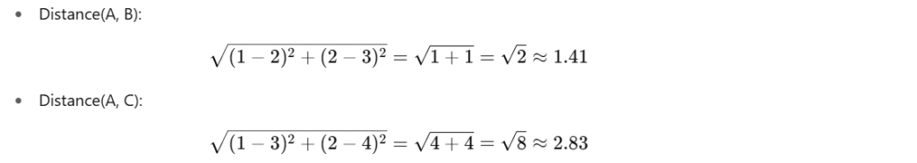
Step 2: Apply distance-weighted average

B’s F3 = 4, Distance = 1.41 → Weight = 1 / 1.41 ≈ 0.71
C’s F3 = 6, Distance = 2.83 → Weight = 1 / 2.83 ≈ 0.35

Imputed F3 for A = 4.66

Python Implementation:

from sklearn.impute import KNNImputer
import pandas as pd
import numpy as np

data = {
‘F1’: [1, 2, 3],
‘F2’: [2, 3, 4],
‘F3’: [np.nan, 4, 6]
}
df = pd.DataFrame(data)

imputer = KNNImputer(n_neighbors=2, weights=’distance’)
imputed = imputer.fit_transform(df)
print(pd.DataFrame(imputed, columns=df.columns).round(2))

When to Use Which Distance?

Distance Metric	Best For	Notes
Euclidean	Continuous data, scaled features	Default in KNN
Manhattan	Sparse data, robust to outliers	Linear paths
Minkowski (p=1.5~3)	Tunable for different behaviors	More control
Cosine	Text data, high-dimensional vectors	Ignores magnitude
Hamming	Binary/categorical features	For classification/imputation

Note: By default, KNNImputer in scikit-learn only supports Euclidean distance (actually the squared Euclidean distance) — and they don’t give you a metric parameter like KNeighborsClassifier does.

So, if you want Manhattan, Hamming, Cosine, etc., you basically have other options:

• Implement a Custom KNN Imputer from Scratch
• Wrap KNNImputer in a Custom Class with Precomputed Distances
• Use fancyimpute or Other Libraries