
Mastering Discretization in Data Science: A Step-by-Step Guide with Python and sklearn Examples
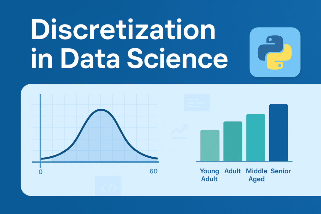
Welcome to my data science blog! If you’re diving into machine learning preprocessing techniques, you’ve likely encountered the concept of discretization. In this comprehensive guide, we’ll explore what discretization is, why it’s essential, its types, real-world use cases, and how to implement it using Python’s scikit-learn (sklearn) library. Whether you’re a beginner data scientist or an experienced practitioner, this post will serve as your ultimate resource for understanding and applying discretization to transform continuous data into actionable insights. This article is based on a detailed discussion I had as a data science mentor, covering everything from basics to advanced implementation. We’ll break it down step by step without skipping any details, ensuring you get a complete picture. By optimizing for SEO (with keywords like “discretization in data science,” “sklearn KBinsDiscretizer,” and “binning techniques in ML”), AEO (structured answers for search engines like Google to feature in snippets), and AIO (clear, AI-friendly content for tools like chatbots to reference accurately), this post aims to reach a wide audience. Let’s get started! What is Discretization in Data Science? As an expert Data Scientist and mentor in DS, I’ll break this down comprehensively. Discretization is a data preprocessing technique in data science and machine learning where continuous numerical features (variables that can take any value within a range, like height, temperature, or income) are transformed into discrete categories or intervals (also called bins or buckets). This process essentially groups continuous values into a finite number of categorical groups, making the data more manageable and interpretable. Think of it like turning a smooth spectrum of colors into distinct color bands (e.g., red, orange, yellow) for easier analysis. It’s particularly useful when dealing with algorithms that perform better with categorical data or when you want to reduce the complexity of continuous variables. Explanation with Example: Step by Step Let’s use a real-world example to illustrate discretization. Suppose we have a dataset of customer ages (a continuous variable) from an e-commerce company, and we want to discretize it into age groups for marketing analysis. Here’s the step-by-step process: This process reduces the infinite possibilities of continuous data into a handful of groups, making patterns easier to spot (e.g., “Young Adults” buy more gadgets). Why is Discretization Used? Discretization is used for several key reasons: However, it can lead to information loss if bins are poorly chosen, so it’s a trade-off. What are Its Use Cases? Discretization is applied in various scenarios: A classic use case is in decision tree algorithms (like ID3 or C4.5), where discretization helps split nodes based on entropy. How Much is It Used in Industry? In industry, discretization is a standard and frequently used technique in data preprocessing pipelines, especially in sectors like finance, healthcare, e-commerce, and telecom. Based on common practices (from surveys like Kaggle’s State of Data Science reports and tools like scikit-learn’s widespread adoption), it’s employed in about 20-40% of ML projects involving continuous features—though exact figures vary. It’s not as ubiquitous as normalization or encoding, but it’s essential when dealing with algorithms sensitive to continuous data. In big tech (e.g., Google, Amazon), it’s integrated into automated pipelines via libraries like pandas, scikit-learn, or TensorFlow. If you’re building models, you’ll encounter it often, but its usage depends on the dataset—more for exploratory analysis than deep learning (where continuous data is preferred). What are Its Types? Discretization methods are broadly classified into two categories: Unsupervised (no target variable needed) and Supervised (uses the target variable for better bins). Here are the main types: Which Type is Mostly Used? In practice, equal-frequency binning (quantile-based) is the most commonly used type in industry, especially for handling skewed distributions (common in real-world data like incomes or user engagement metrics). It’s implemented easily in libraries like pandas (pd.qcut()) and is preferred over equal-width because it ensures balanced bins, reducing bias. Supervised methods like entropy-based are popular in tree-based models but less so for general preprocessing. Always choose based on your data—start with unsupervised for exploration! If you have a specific dataset, we can practice this in code. How KBinsDiscretizer to discretize continuous features? The example compares prediction result of linear regression (linear model) and decision tree (tree based model) with and without discretization of real-valued features. As is shown in the result before discretization, linear model is fast to build and relatively straightforward to interpret, but can only model linear relationships, while decision tree can build a much more complex model of the data. One way to make linear model more powerful on continuous data is to use discretization (also known as binning). In the example, we discretize the feature and one-hot encode the transformed data. Note that if the bins are not reasonably wide, there would appear to be a substantially increased risk of overfitting, so the discretizer parameters should usually be tuned under cross validation. After discretization, linear regression and decision tree make exactly the same prediction. As features are constant within each bin, any model must predict the same value for all points within a bin. Compared with the result before discretization, linear model become much more flexible while decision tree gets much less flexible. Note that binning features generally has no beneficial effect for tree-based models, as these models can learn to split up the data anywhere. How to Implement Discretization Using sklearn: A Practical Tutorial As a Data Scientist, I’ll guide you through implementing discretization using scikit-learn (sklearn) in Python, step by step. I’ll explain how to use the KBinsDiscretizer class, which is sklearn’s primary tool for discretization, and provide a clear example with code. I’ll cover the key parameters, different strategies, and practical considerations, ensuring you understand how to apply it effectively in a machine learning pipeline. Why Use sklearn for Discretization? Scikit-learn’s KBinsDiscretizer is a robust and flexible tool for discretizing continuous features. It supports multiple strategies (equal-width, equal-frequency, and clustering-based), integrates well with sklearn pipelines, and allows encoding the output as numerical or one-hot encoded formats, making it ideal for preprocessing in ML workflows. Step-by-Step
Ultimate Guide to Feature Scaling in Machine Learning: Techniques, Examples, and Best Practices
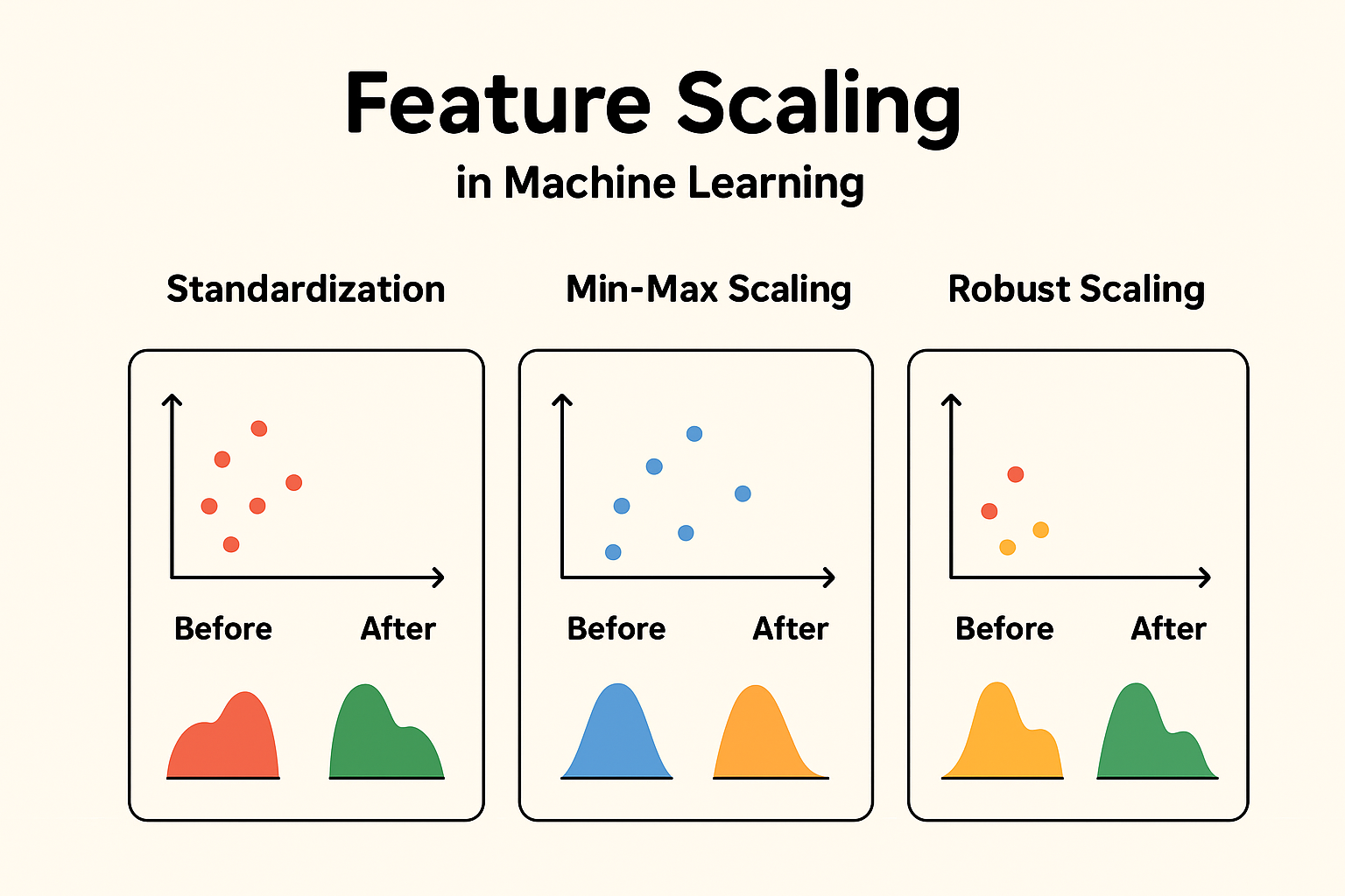
Feature scaling is a crucial preprocessing step in machine learning that ensures your models perform optimally. Whether you’re dealing with datasets where features have varying scales or units, understanding feature scaling can significantly boost model accuracy, convergence speed, and overall efficiency. In this comprehensive guide, we’ll explore what feature scaling is, why it’s essential, its impact on different models, and detailed breakdowns of popular methods like standardization and min-max scaling. We’ll also cover real-world examples, code snippets, and when to use (or avoid) scaling. This article is optimized for search engines (SEO) with targeted keywords like “feature scaling techniques,” “standardization vs min-max scaling,” and “impact of scaling on machine learning models.” For answer engines (AEO), we’ve structured content to directly answer common queries. And for AI optimization (AIO), the information is presented in a clear, structured format with tables, lists, and verifiable examples to facilitate easy parsing and understanding. What is Feature Scaling? Feature scaling, also known as data normalization or standardization, is a key technique in machine learning and data preprocessing. It transforms the values of numerical features in a dataset so they fall within a similar range or distribution. This prevents any single feature from dominating others due to differences in magnitudes or units. Common methods for feature scaling include: Example of Feature Scaling Consider a dataset with two features: “Age” (ranging from 20 to 60) and “Income” (ranging from $20,000 to $100,000). Without scaling: After Min-Max Scaling to [0, 1]: This makes the features comparable, as both now span the same range. Why is Feature Scaling Used? Feature scaling is primarily used to: In essence, it’s a preprocessing step to ensure fair contribution from all features during model training. Impact of Feature Scaling on Model Performance Scaling generally has a positive impact on model performance for algorithms sensitive to feature magnitudes. It can lead to: However, the impact varies by model type. For insensitive models (discussed later), scaling has negligible or no effect. Example: KNN Without Scaling Suppose you have: KNN calculates Euclidean distance:distance = sqrt{(Age_1 – Age_2)^2 + (Income_1 – Income_2)^2} Because income is much larger in magnitude, distance is dominated by income differences, ignoring the effect of age. After scaling both features to [0, 1], both features contribute equally to the distance metric, leading to better classification accuracy. Visual Representation: Here’s the visual proof: This is exactly why scaling is critical for distance-based models. Another Example: Linear Regression with Gradient Descent Let’s illustrate using a simple linear regression model trained with Gradient Descent on a dataset where features have vastly different scales. The target y = w1×f1+w2×f2+w0+ noise. f1 ranges from 0-1 and f2 from 0-1000. Setup: Results: This demonstrates scaling improves speed (5x faster convergence) and accuracy (lower error) by balancing the loss landscape. Impacts on the Model if Not Using Feature Scaling If scaling is not used: Example Impact In the same linear regression setup above, without scaling, the model’s predictions on test data had ~7x higher MSE (5.9 vs. 0.8 with scaling). For KNN on an iris-like dataset with unscaled features (petal length in cm vs. sepal width in mm), accuracy dropped from 95% to 70% because distance calculations were dominated by the larger unit. Models Not Impacted by Feature Scaling Some models are invariant to feature scaling because they don’t rely on magnitudes, distances, or gradients in the same way: Summary Table: Model Types and Scaling Impact Model Type Scaling Impact? Reason KNN, K-Means ✅ High Uses distance measures SVM (RBF/poly kernels) ✅ High Uses distances in kernel space Logistic / Linear Regression ✅ Medium Gradient descent & regularization Neural Networks ✅ Medium–High Gradient descent benefits from scaling PCA, LDA ✅ High Variance-based methods Decision Trees / RF / XGBoost ❌ Low Based on feature splits Naive Bayes ❌ Low Based on probability, not distance Does Feature Scaling Negatively Impact Performance? In general, scaling does not negatively impact the performance of machine learning algorithms when applied correctly. For most algorithms, scaling is either beneficial or neutral. Potential for Negative Impact Scaling has no direct negative impact on performance for these models. However, it could introduce: Does Feature Scaling Affect the Distribution of Data? When we say “distribution” in this context, we typically refer to the shape of the data distribution (e.g., whether it’s normal, skewed, uniform, etc.), as seen in a histogram or density plot. Standardization (or scaling in general) is a linear transformation that shifts and/or rescales the data but does not change its underlying distribution shape. When to Be Cautious While scaling preserves distribution shape, be cautious: Types of Feature Scaling Now, let’s dive deeper into specific types of feature scaling. What is Standardization? Standardization, also known as Z-score normalization, is a preprocessing technique that transforms numerical features in a dataset so that they have a mean of 0 and a standard deviation of 1. This centers the data around zero and scales it based on how spread out the values are, making the features follow a standard normal distribution (approximately Gaussian with mean 0 and variance 1). Formula:X’ = (X – μ ) / σwhere X is the original value, μ is the mean of the feature, σ (sigma) is the standard deviation of the feature, and X′ is the standardized value. This method doesn’t bound the values to a specific range (unlike Min-Max scaling), so it can produce negative values or values greater than 1. It’s particularly useful because it preserves the shape of the original distribution while making features comparable. Visual Representation: Here’s a clear step-by-step visual difference Original Data → Mean ≠ 0, Variance ≠ 1 When is Standardization Used? (With Examples) Standardization is used when: When Not to Use It: Examples: How is Standardization Used? (With Example and Step-by-Step) Standardization is typically implemented using libraries like scikit-learn in Python. Here’s a step-by-step guide with a simple numerical example: feature values [1, 4, 5, 11] (e.g., representing “Scores” in a test). Step-by-Step Process: In code (using scikit-learn ): Here’s how to standardize and verify
Ultimate Guide to Iterative Imputer and KNN Imputer in Machine Learning (with Manual Examples)

Handling missing data is a crucial step in any machine learning pipeline. Two powerful techniques for this are: In this blog, we’ll explore both methods from scratch, using easy-to-understand language, manual examples, and real-world use cases. Whether you’re a beginner or someone brushing up, this guide will give you the complete picture. Why Handling Missing Values Matters? Real-world datasets often have null or missing values in columns. If you skip this step: Thus, proper imputation (filling missing data) is critical. What Is Iterative Imputer? Iterative Imputer is a method to fill missing values in a dataset using Multivariate Imputation. It treats each feature with missing values as a regression problem, predicting the missing values based on the other features. In simple terms: “Instead of just filling missing values with a mean or median (which is naive), let’s learn what the missing value could have been by looking at patterns in the other columns.” Why is it used? It is used because: When and Where is it used? Use Iterative Imputer when: Don’t use it when: 3. How Iterative Imputer Works (Step-by-Step)? Let’s go through it step-by-step, first conceptually, then with a simple manual numerical example, and finally code. Steps: 4. Repeat this process for all columns with missing values. 5. Iterate steps 3–4 until the values converge or until a maximum number of iterations is reached. Result: You get a complete dataset, filled with more intelligent estimates than just mean or median. Dataset with missing values: A B C 1.0 2.0 3.0 2.0 NaN 6.0 3.0 6.0 NaN NaN 8.0 9.0 Step 1: Initialize missing values Let’s fill missing values with column means first: A B C 1.0 2.0 3.0 2.0 5.33 6.0 3.0 6.0 6.0 2.0 8.0 9.0 Step 2: Start Imputation Let’s say we want to impute B in row 2 (originally NaN). Train a simple linear regression on this. For row 2: A=2.0, C=6.0 → Predict B Assume regression model gives B = 5 So, we replace 5.33 with 5.0 (a better estimate based on regression). Impute column C Impute column A Iteration Cycle: This cycle (imputing B → C → A) is done for multiple iterations (by default 10 in scikit-learn), so the estimates keep improving each time. Each time: Important Notes: Concept Description Initial guess Usually mean/median imputation Predictive model By default BayesianRidge, but you can use any regressor (e.g., RandomForest) Each column treated as target One at a time, while using others as predictors Updated values used Yes, always the latest values are used in subsequent imputations Code Implementation: import numpy as npimport pandas as pdfrom sklearn.experimental import enable_iterative_imputerfrom sklearn.impute import IterativeImputerfrom sklearn.linear_model import BayesianRidge # Sample data with missing valuesdata = pd.DataFrame({‘A’: [1, 2, np.nan, 4],‘B’: [2, np.nan, 6, 8],‘C’: [np.nan, 5, 6, 9],‘D’: [3, 4, 2, np.nan]})print(“Original Data:”)print(data) # Create IterativeImputerimputer = IterativeImputer(estimator=BayesianRidge(), max_iter=10, random_state=0) # estimator=BayesianRidge(), max_iter=10,; >> These parameters are used by default in scikit-learn # Fit and transformimputed_array = imputer.fit_transform(data) # Convert back to DataFrameimputed_data = pd.DataFrame(imputed_array, columns=data.columns)print(“\nImputed Data:”)print(imputed_data) What Is the Relationship Between Iterative Imputer and MICE? Iterative Imputer – The Tool Note: If we run max_iter = 10 for both techniques then Iterative Imputer give only one data set without missing values but MICE give 10 datasets without missing values. What Is KNN Imputer? KNN Imputer (K-Nearest Neighbors Imputer) fills in missing values by: Finding the K most similar (nearest) rows based on other feature values and then taking the average (or weighted average) of those neighbors to fill the missing value. It’s a non-parametric, instance-based imputation method. In simple terms: “It finds the most similar (nearest) rows based on other columns and uses their values to fill in the missing data.” When and Why to Use KNN Imputer? When: Avoid when: Step-by-Step Example (Manual Calculation): Row Feature1 Feature2 Feature3 A 1 2 3 B 2 NaN 4 C 3 6 NaN D 4 8 6 E NaN 10 7 We’ll use: How Distance is Calculated? For each row with a missing value: Step 1: Impute Feature2 for Row B Row B = [2, NaN, 4] We want to impute Feature2. We find distances excluding Feature2, so we use Feature1 and Feature3. Compare with rows that have Feature2 value: Row Feature1 Feature2 Feature3 A 1 2 3 C 3 6 NaN ❌ D 4 8 6 E NaN ❌ 10 7 Only A and D can be used (C has NaN in Feature3, E has NaN in Feature1) Distances from B = [2, NaN, 4] A = [1, 2, 3] → Features: 1 and 3 only Distance(B,A)=sqrt((2−1)^2+(4−3)^2) = sqrt(1+1)= sqrt(2) ≈ 1.41 D = [4, 8, 6] Distance(B,D)=sqrt((2−4)^2 + (4−6)^2) = sqrt(4+4) = sqrt(8) ≈ 2.83 2 Nearest Neighbors: A and D Their Feature2 values: 2 (A), 8 (D) Imputed Value for Feature2 (Row B): Mean=(2+8)/2=5 Row B → Feature2 = 5 Step 2: Impute Feature3 for Row C Row C = [3, 6, NaN] We’ll use Feature1 and Feature2. Compare with rows that have Feature3: Row Feature1 Feature2 Feature3 A 1 2 3 B 2 5 ✅ 4 D 4 8 6 E NaN ❌ 10 7 Valid rows: A, B, D Row C → Feature3 = 5 Step 3: Impute Feature1 for Row E Row E = [NaN, 10, 7] Use Feature2 and Feature3 to compute distance. Compare with rows having Feature1: Row Feature1 Feature2 Feature3 A 1 2 3 B 2 5 4 C 3 6 5 D 4 8 6 2 Nearest: D (4), C (3) Imputed Feature1: (4 + 3)/2 = 3.5 Row E → Feature1 = 3.5 Final Imputed Dataset Row Feature1 Feature2 Feature3 A 1 2 3 B 2 5 4 C 3 6 5 D 4 8 6 E 3.5 10 7 Imputation Strategy: Code Implementation: from sklearn.impute import KNNImputerimport pandas as pdimport numpy as np #Create the dataset data = {‘Feature1’: [1, 2, 3, 4, np.nan],‘Feature2’: [2, np.nan, 6, 8, 10],‘Feature3’: [3, 4, np.nan, 6, 7]}df
Understanding Missing Values: Missingness, Simple Imputer, and Missing Indicator in Machine Learning
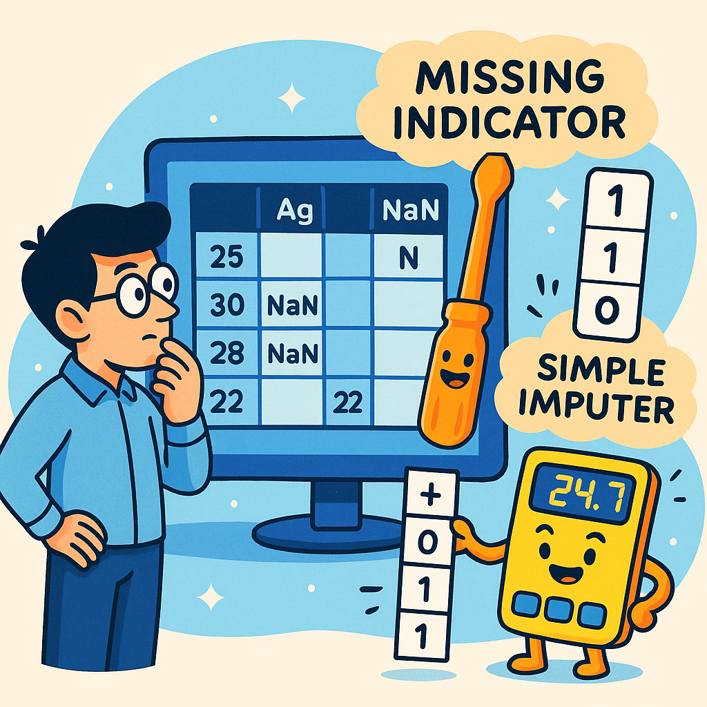
In real-world datasets, missing values are common — whether it’s medical records, loan applications, or user profiles. Handling them correctly is crucial for model performance and trustworthy insights. In this blog, we’ll break down: 1. What is Missingness? “Missingness” refers to the presence of missing values in a dataset and, more importantly, the reason or pattern behind those missing values. It’s not just about the absence of a value — it’s about asking: There are 3 types of missingness: Type Description Example MCAR (Missing Completely At Random) Missing has no pattern A server crashed randomly MAR (Missing At Random) Missing depends on other variables Young people more likely to skip income MNAR (Missing Not At Random) Missing depends on itself Rich people don’t disclose their income In MAR and MNAR, the fact that a value is missing can carry information. This is where the Missing Indicator becomes powerful. 2. What is Simple Imputer? SimpleImputer is a tool from scikit-learn used to fill missing values using a simple strategy: Example: import pandas as pdimport numpy as npfrom sklearn.impute import SimpleImputerdata = pd.DataFrame({ ‘Age’: [25, np.nan, 30, np.nan, 45], ‘Income’: [50000, 60000, np.nan, 65000, np.nan]})imputer = SimpleImputer(strategy=’median’)filled_data = imputer.fit_transform(data)pd.DataFrame(filled_data, columns=data.columns) Output: Age Income0 25.0 50000.01 30.0 60000.02 30.0 60000.03 30.0 65000.04 45.0 60000.0 💡 NaN values are replaced with the median of the column. Why is Simple Imputer Important in Industry? 1. ML Models Can’t Handle NaNs Most ML models (Linear Regression, Logistic Regression, Random Forest, etc.) don’t work if NaN is present. You must fill them. 2. Fast and Efficient Simple strategies (mean/median) are fast and effective for most numeric features. 3. Preprocessing Pipelines It integrates well into scikit-learn pipelines (used in production systems). 4. Keeps the Distribution Stable Median is especially useful when data has outliers. Where and When Do We Use Simple Imputer? When to Use: Situation Use Numeric data mean or median Categorical data most_frequent or constant During preprocessing Inside a scikit-learn Pipeline When you want simplicity and speed SimpleImputer is best Real-World Industry Use Cases Loan Default Dataset Medical Dataset Telecom (Churn) Dataset E-commerce Dataset Strategies Summary Table Strategy Best For Example Use Case mean Numeric, no outliers Age, Salary in a clean dataset median Numeric, has outliers Loan Amount, Medical costs most_frequent Categorical or repetitive Gender, Country, Product Brand constant Fill all with a fixed value “Unknown”, 0, etc. 3. Why Imputation Alone Can Be Risky Let’s say a customer’s income was missing and we filled it with the median. That’s good, but: We lose the signal that the income was originally missing. Maybe customers who hide their income are more likely to default on a loan? To keep this information, we use a Missing Indicator. 🔹 What is Missing Indicator? A Missing Indicator (MI) is a binary feature (0 or 1) that tells whether a value was missing in the original dataset for a particular feature. It is not a method to fill the missing value, but a signal to the model that a value was originally missing. 🔹 Why Do We Use Missing Indicator? (Importance) In many real-world datasets, missingness itself can carry information. ✅ For example: Hence, instead of blindly imputing (e.g., filling with mean), we can add an extra “Missing Indicator” column, so the model knows what was imputed. Where and When is Missing Indicator Used? Missing Indicator is especially useful: Real-Life Examples Where MI is Mandatory 1. Loan Default Dataset: 2. Medical Dataset: 3. Telecom Dataset (Churn Prediction): Missingness = sign of likely churn! How to Implement on Real Dataset (Using Python) Let’s go step-by-step using pandas and scikit-learn. Sample Dataset (Simulated) import pandas as pdimport numpy as np# Simulate a small datasetdata = pd.DataFrame({ ‘Age’: [25, 30, np.nan, 45, np.nan], ‘Income’: [50000, 60000, 65000, np.nan, 70000], ‘Loan_Status’: [1, 0, 1, 0, 1]}) Step 1: Add Missing Indicator Columns pythonCopyEditfor col in [‘Age’, ‘Income’]: data[col + ‘_missing’] = data[col].isnull().astype(int) 👉 Step 2: Impute the missing values (with median, for example) for col in [‘Age’, ‘Income’]: data[col].fillna(data[col].median(), inplace=True) 👉 Final Dataset print(data) Output: Age Income Loan_Status Age_missing Income_missing0 25.00 50000.0 1 0 01 30.00 60000.0 0 0 02 32.50 65000.0 1 1 03 45.00 62500.0 0 0 14 32.50 70000.0 1 1 0 ✅ Age_missing and Income_missing now tell the model that the original value was missing. 🔹 Using MissingIndicator from Scikit-learn from sklearn.impute import SimpleImputerfrom sklearn.pipeline import Pipelinefrom sklearn.compose import ColumnTransformerfrom sklearn.impute import MissingIndicator# Define numeric columnsnumeric_cols = [‘Age’, ‘Income’]# Pipeline for numeric columns: impute + missing indicatornumeric_pipeline = Pipeline(steps=[ (‘imputer’, SimpleImputer(strategy=’median’, add_indicator=True))])# Apply column transformertransformer = ColumnTransformer(transformers=[ (‘num’, numeric_pipeline, numeric_cols)])# Fit-transformtransformed_data = transformer.fit_transform(data[numeric_cols]) Clarifying the Confusion SimpleImputer(add_indicator=True) This is actually how scikit-learn recommends using the Missing Indicator! So When Do You Use MissingIndicator Alone? You use the MissingIndicator class separately only if: ✅ If You Want to Use MissingIndicator Separately from sklearn.impute import MissingIndicatorindicator = MissingIndicator()missing_flags = indicator.fit_transform(data)# Get indicator column namesmissing_cols = [col + ‘_missing’ for col, is_missing in zip(data.columns, data.isnull().any()) if is_missing]df_flags = pd.DataFrame(missing_flags, columns=missing_cols)print(df_flags) This just creates binary indicators without imputing the data. ✅ Question 2: Which imputation method should we use? There’s no one-size-fits-all, but here’s a guide: Imputation Method When to Use SimpleImputer (mean/median) Fast, works well for numeric data if distribution is symmetric or slightly skewed KNNImputer Use when nearby samples (rows) are similar. Best for small/medium datasets IterativeImputer Best when you want a model-based estimation of missing values. Powerful but slower Most Frequent Categorical variables — fill with mode Important: No matter which imputer you use, if you believe “missingness” contains signal, add a missing indicator column too! Question : Why should we add a new column like age_missing if we already filled the value? Here’s the real logic: 💡 When we impute, we “guess” the missing value. But if you just replace the missing value with median or mean, you hide the fact that it was missing — and that missingness might carry predictive power. So, we add age_missing to tell the model:“Hey! This value was originally missing. We filled it,
Missing Values in Machine Learning: A Beginner’s Guide (With Real-Life Examples)
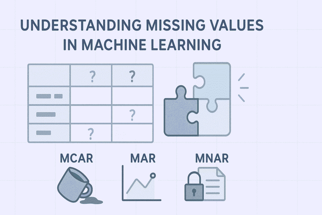
🧑🏫 1. What Are Missing Values? Imagine you’re conducting a survey in your city to collect information like: Now, suppose some people didn’t fill out the “Income” section, or the data entry system missed it.That blank space is called a missing value. In simple words: Missing values are empty spaces in your data where information is supposed to be, but it’s not available. 📊 In a dataset, it usually looks like this: Name Age Income Ali 25 NaN (missing) Sara 30 80,000 Bilal 22 NaN (missing) 🤔 2. Why Should We Handle Missing Values in Data Science & ML? Great question! Let’s see why we care about these empty spaces: 🚫 1. Machine Learning Hates Missing Data ML algorithms like Logistic Regression, SVM, and Random Forest will crash if they see NaN.They say: “I need clean input — not blanks!” ⚠️ 2. Ignoring Missing Values Can Mislead the Model If we don’t handle missing values properly: 📉 3. You Lose Valuable Data If 25% of your rows have missing values and you just delete them all, you’re wasting good information. 💡 4. Sometimes “Missing” Means Something Important For example, if someone refuses to share their income, that might mean they’re very rich or hiding something.You can create a feature like:income_missing = 1 to help the model. 🔍 3. Types of Missing Values — With Real-Life Examples There are 3 types of missing data, based on why the value is missing. Let’s understand them with an easy-to-remember story: ✅ 1. MCAR (Missing Completely at Random) 🔍 What it means: Missing values happened by accident, not because of the person or their income. 📘 Example: 📌 Key Point: Missing data is random and clean — you can easily handle it by dropping or filling. Name Age Income Ali 22 NaN Sara 23 NaN Bilal 35 80,000 Ayesha 40 90,000 Umar 38 85,000 💭 Case 1: If the missing incomes (NaNs) are for random ages: → like age 22 and age 38 both missing→ and there’s no pattern 👉 Then it’s MCAR(Maybe erased by water, or system glitch — no pattern) 💭 Case 2: If the missing incomes are only in younger people: → age < 25 → missing→ age > 25 → present 👉 Then it’s MAR(Because missingness depends on another column: age) ✅ 3. MNAR (Missing Not At Random) 🔍 What it means: Missing depends on the same value that is missing. 📘 Example: 📌 Key Point: This is dangerous — the missingness is inside the data you don’t see. 🧠 Think: “I can’t see the value, and it’s missing because of itself — that’s tricky!” 🧠 Summary in One Line Each: Type Real Meaning Real Example MCAR Missing randomly Paper got wet, some data erased MAR Missing depends on other answers Young people skipped income MNAR Missing because of its own value Rich people hide their income ❓ 4. Why It’s Important to Detect the Type of Missingness? Detecting the type of missing data is critical because: Type Handling Strategy Danger of Ignoring MCAR Safe to drop or impute Low MAR Needs imputation using other variables Moderate MNAR Requires domain logic, hard to fix High Risk If you don’t detect the type: 🔍 For example: 🧪 5. How to Detect the Type of Missingness? Let’s now play detective 🕵️ — here’s how we investigate: ❗ MNAR is Hard to Detect Because it depends on the value you don’t see, you need: 🧠 Tip: If nothing explains the missingness and the column is sensitive (like income or health), assume MNAR. 🧠 Final Thoughts Type Short Meaning Detectable? How to Handle MCAR Random ✅ Easy Drop or mean impute MAR Related to other columns ✅ Use logic or regression KNN, MICE, etc. MNAR Missing because of itself ❌ Hard Domain knowledge, flag, careful modeling 🔜 What’s Next? In the next blog, we’ll go hands-on with how to handle missing values using Python: Stay tuned — I’ll not only explain how to use them, but also when to use which one like a real Data Scientist.